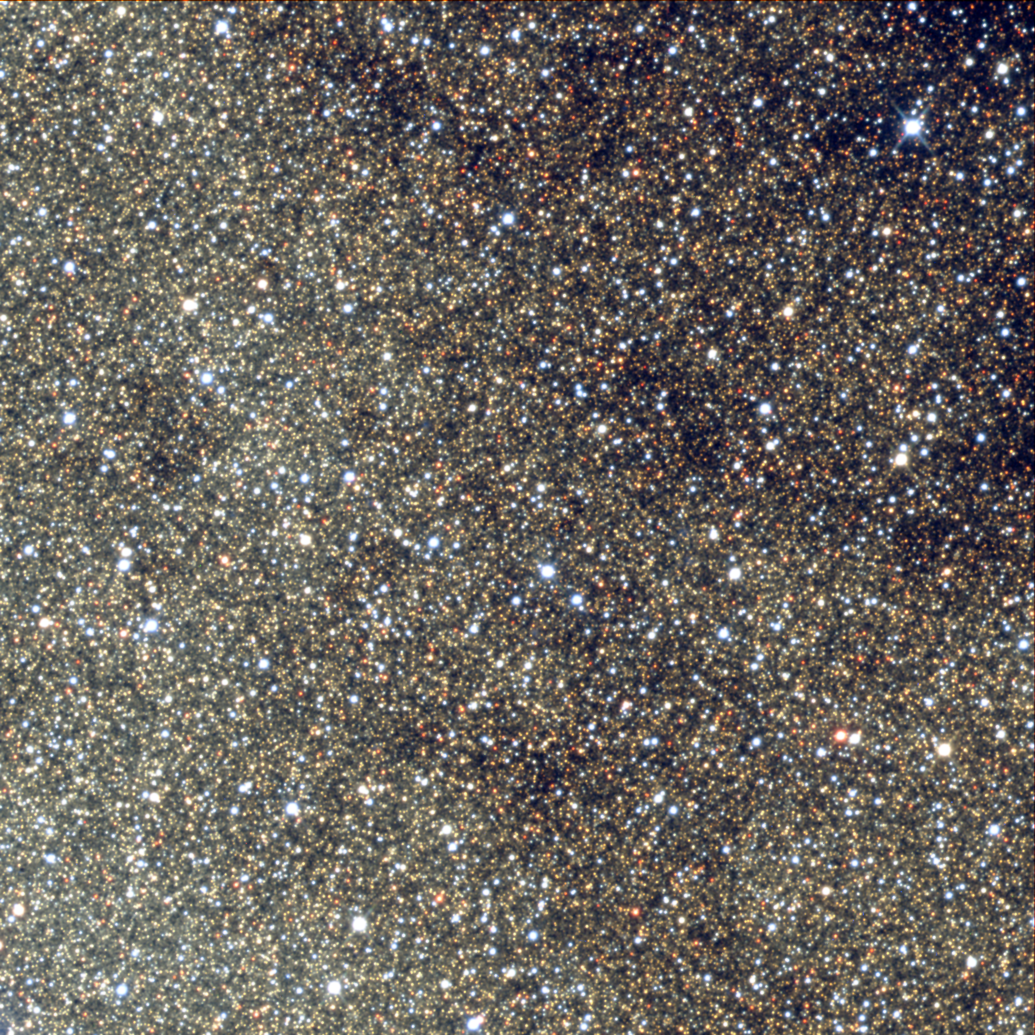
Photometry in crowded fields

<p>Microlensing is an inherently rare phenomenon, so we need to monitor millions of stars in order to detect events. <p> <p>→ Monitor densely populated regions of the sky, e.g. the Galactic Bulge. </p> <p>So microlensing is most often detected in crowded starfields.</p> <br> <p><small>The field of OGLE-2012-BLG-0406 (centered)<br>

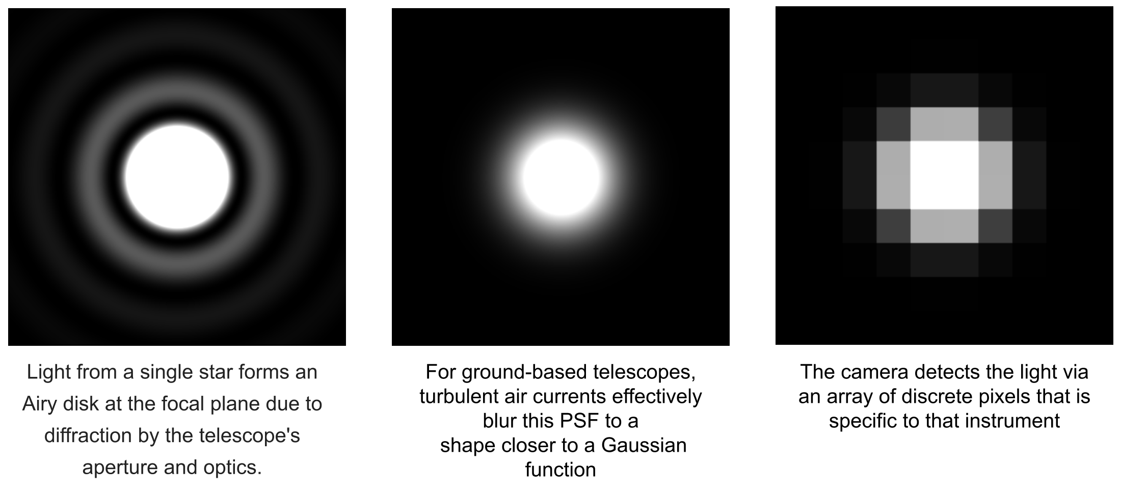
Point Spread Functions (PSF)

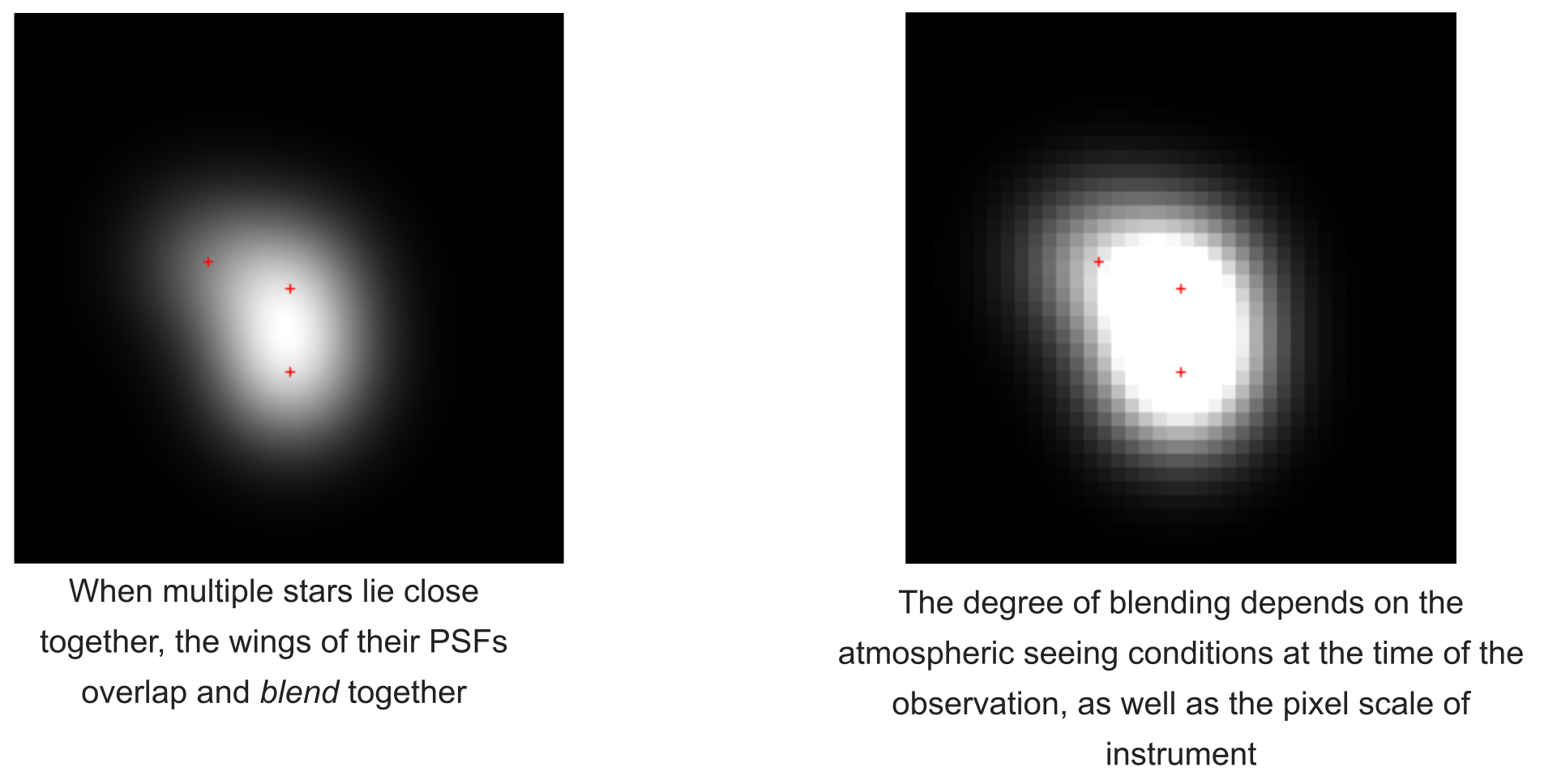
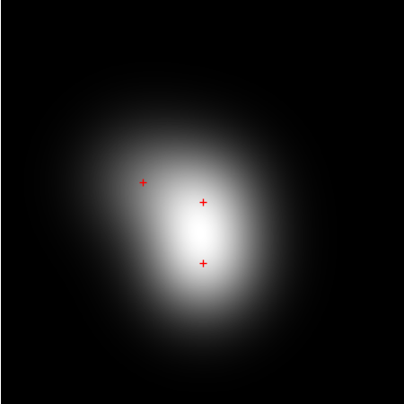
Blended Point Spread Functions

Measuring Flux

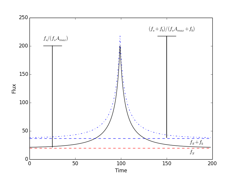
Blending results in light from the neighbors contaminating the flux of the lensed star, f_λ,s, measured at time t.

Isolated lensed star:

$$f_{\lambda}(t) = f_{\lambda,s}(t)A(u(t))$$

Blended star:

$$f_{\lambda}(t) = f_{\lambda, s}(t)A(u(t)) + f_{\lambda, b}(t)$$

where f_λ(t) = measured flux, A(u(t)) = magnification at angular separation u, and f_b(t) = blend flux. You may also see the blend ratio, g = f_b/f_s.

This is strongly time and wavelength dependent - so f_s, f_b are measured for each dataset

Blending in microlensing light curves

Blending can make t_E appear shorter, leading to a mis-estimation of the lens parameters.

It can be a symmetrical change in the light curve, mimicing the parallax component π_E,⊥.

Dealing with Blending

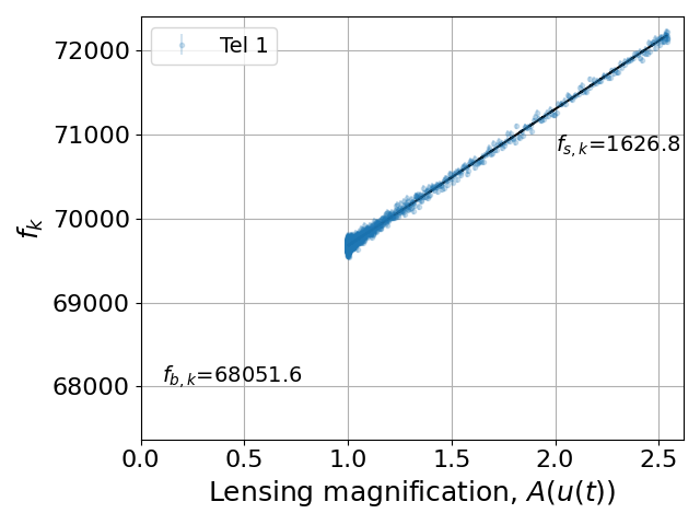
Only the source star is magnified, and A(u(t)) can usually be considered to be the same for all observers.

By measuring the total flux as a function of time for each telescope, we can find the best-fit model for A(u(t)) that includes both source and blend fluxes.

Further reading

• Alcock, C. et al. (1997), ApJ, 479, 119
• Wozniak, P & Paczyński,B. (1997), ApJ, 487, 55
• Han, C.(1999), MNRAS, 309, 373