So far we have considered the lens to be a single massive object, but if a companion is present in the lens system, the result can be complex and beautiful microlensing light curves.
Understanding binary lenses is the key to the discovery of planetary systems through microlensing.Outline
- Blending
- Finite source effects
- Binary lensing
Photometry in crowded fields
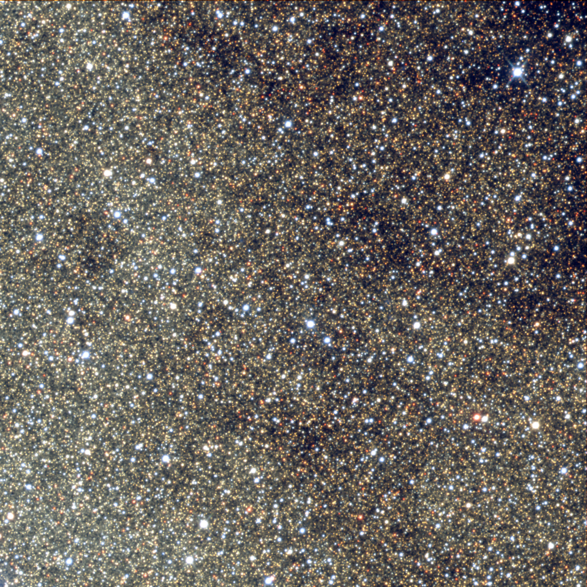
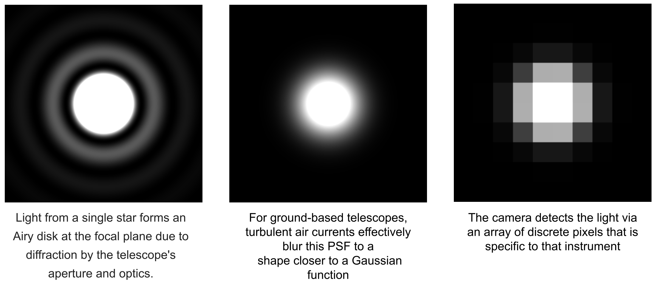
Point Spread Functions (PSF)
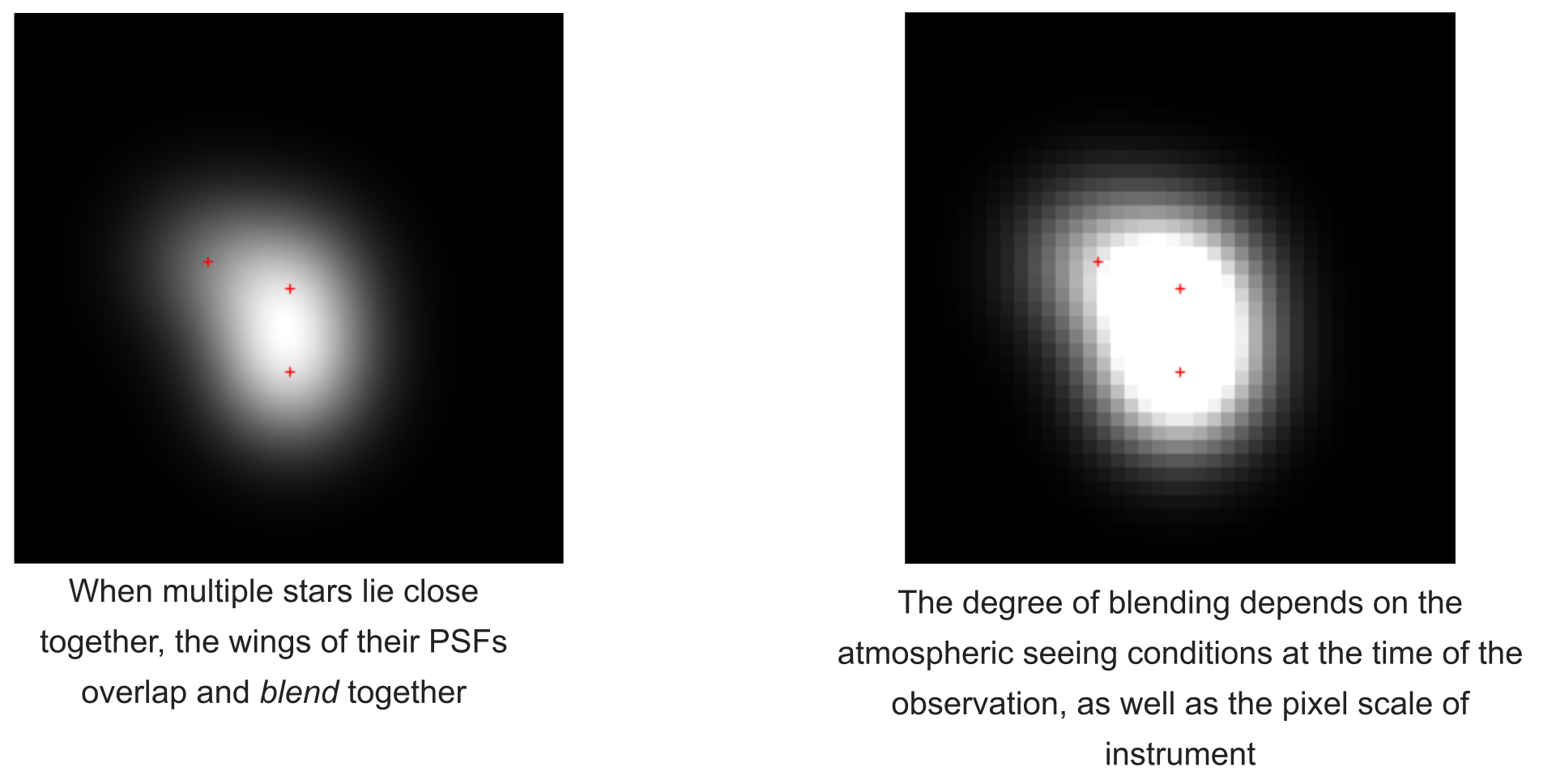
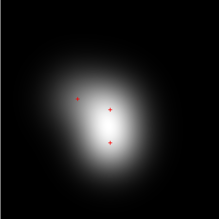
Blended Point Spread Functions
Measuring Flux
Blending results in light from the neighbors contaminating the flux of the lensed star, fλ,s, measured at time t.

Isolated lensed star:
$$f_{\lambda}(t) = f_{\lambda,s}(t)A(u(t))$$
Blended star:
$$f_{\lambda}(t) = f_{\lambda, s}(t)A(u(t)) + f_{\lambda, b}(t)$$
where fλ(t) = measured flux, A(u(t)) = magnification at angular separation u, and fb(t) = blend flux. You may also see the blend ratio, g = fb/fs.
This is strongly time and wavelength dependent - so fs, fb are measured for each dataset
Blending in microlensing light curves
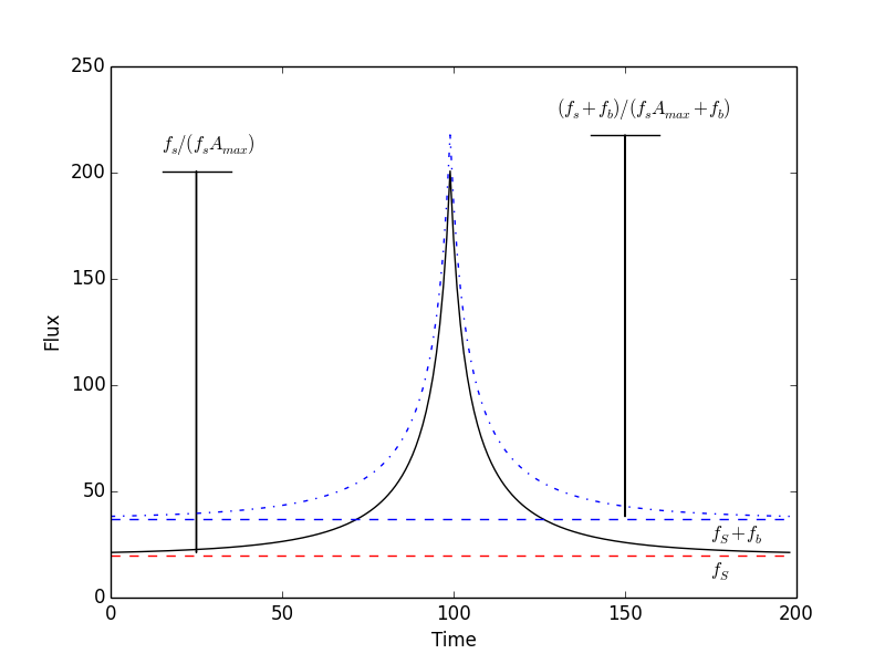
Blending can make tE appear shorter, leading to a mis-estimation of the lens parameters.
It can be a symmetrical change in the light curve, mimicing the parallax component πE,⊥.
Dealing with Blending
We need observations at a range of different magnifications
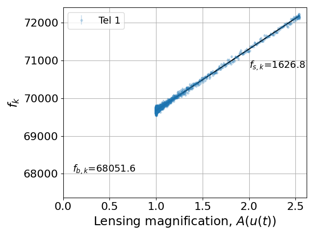
Only the source star is magnified, and A(u(t)) can usually be considered to be the same for all observers.
By measuring the total flux as a function of time for each telescope, we can find the best-fit model for A(u(t)) that includes both source and blend fluxes.
Further reading
Introduction
Generally in astronomy its pretty safe to treat them as point sources given their enormous distances!
But microlensing is an extraordinarily sensitive technique and even the radius of a star almost half way across the Galaxy can have a measureable effect.
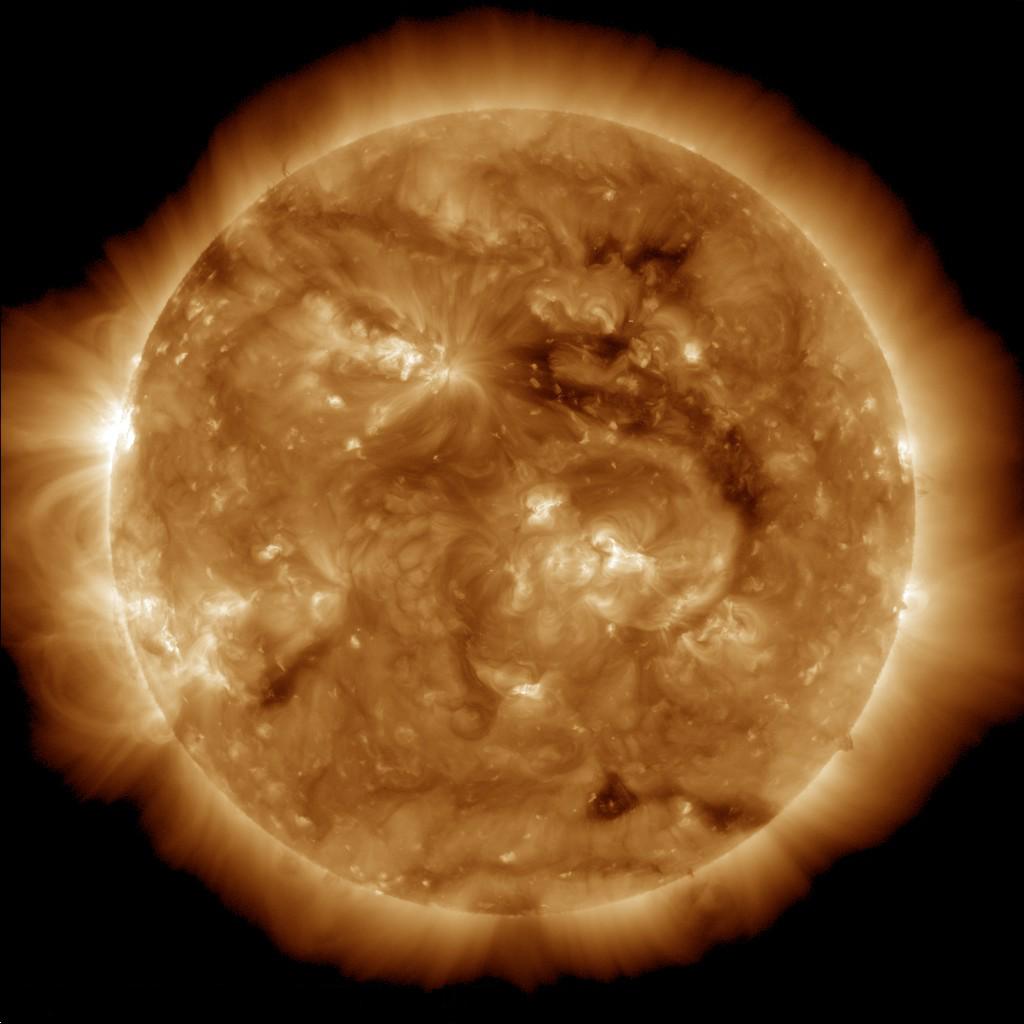
Image credit: JPL/NASA Solar Dynamic Observatory
Lens and Source Planes
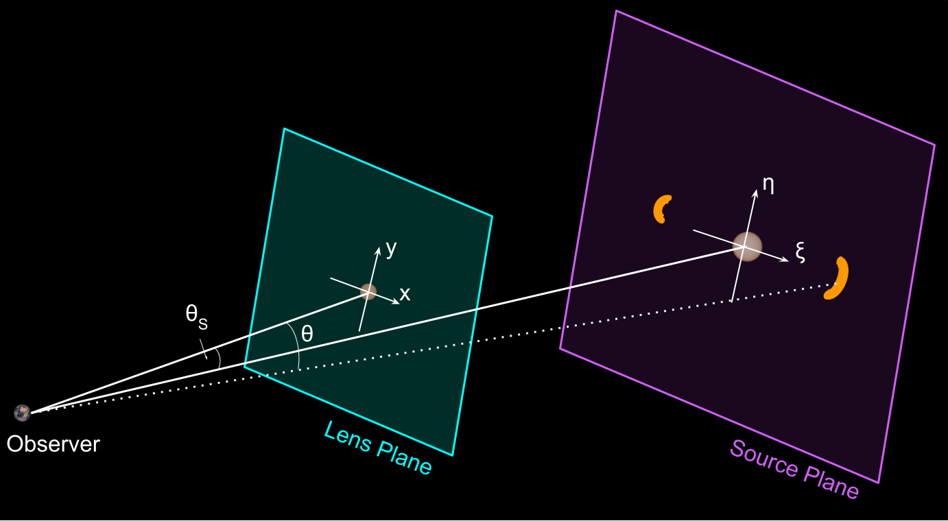
Lensing can be thought of as a 'mapping' of the coordinate system in the lens plane (x,y, centered on the lens) to that of the source (ξ,η).
θ1,2 = angular offsets of source images
θE = angular Einstein radius
θ = angular separation between lens and source
Sources of Finite Extent
Within these reference frames, we need a way to represent the finite disk of the source star, including its radial brightness profile.
RS = source star physical radius
θ* = source star angular radius
ρ = θ* normalized by the angular Einstein radius θE
The Lens Equation (again)
Here we introduce complex notation in order to parameterize the lens equation.
This provides a more natural formulation for two-dimensional vectors. Much of this theory was originally explored in the context of lensed quasars and other large-scale masses.
$$\zeta = \xi + i\eta$$
$$z = x + iy,$$
where z and ζ are normalized to the Einstein radius in the lens, source planes respectively.
The Lens Equation
The equation for a single lens can then be re-written:
$$\zeta - \frac{D_{S}}{D_{L}}z - D_{LS}\alpha(z,\bar{z}) = 0,$$
where α is the complex deflection angle α(z, z̄) = αx(x, y) + iαy(x, y) and z̄ is the complex conjugate of z.
The solutions of this form of the lens equation are then:
$$z_{1,2} = \frac{\xi}{2}\left( 1 \pm \sqrt{1 + \frac{4}{\zeta\bar{\zeta}}} \right)$$
See Witt 1990, Witt & Mao 1994 and Mao & Witt 1998 for a full derivation of finite-source expressions.
Sources of Finite Extent
In this notation a single, circular source of finite radius r can be described as:
$$\zeta(\phi) = \zeta_{0} + re^{i\phi},$$
where φ = θ-2π and ζ0 is the (parameterized) impact parameter. This is simply substituted into the solutions for the lens equations to derive the parameterized image locations:
$$z_{1,2} = \frac{\zeta_{0}+re^{i\phi}}{2}\left[ 1 \pm \sqrt{1 + \frac{4}{\zeta_{0}^{2} + 2r\zeta_{0}\cos{\phi+r^{2}}}} \right],$$
Finite Source Size and Magnification
Since surface brightness is conserved, the magnification (Atot) is given by the ratio of the combined image area to that of the unlensed source.
In complex notation the areas of both images is given by:
$$A_{1,2} = \frac{1}{2\pi r^{2}} \int_{0}^{2\pi} y(\phi) \frac{dx(\phi)}{d\phi},$$
Finite Source Size and Magnification
In these expressions:
$$x(\phi) = \frac{\zeta_{0} + r\cos\phi}{2}f_{1,2}(\phi),$$
$$y(\phi) = \frac{r\sin\phi}{2}f_{1,2}(\phi),$$
$$f_{1,2}(\phi) = 1 \pm \sqrt{1 + \frac{4}{\zeta_{0}^{2} + r^{2} + 2\zeta_{0}r\cos\phi}}$$
Observable Effects
The observable effects of the finite extent of the source are illustrated below.
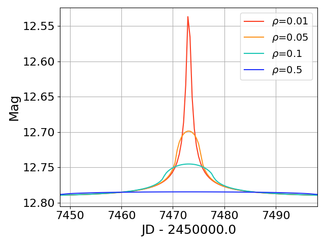
The lightcurve is noticably "rounded-over" at the peak of the event in comparison with the PSPL model, and the amplitude can differ significantly.
These effects become significant when the impact parameter ≈ θ*
In practice this prevents real events from achieving the (theoretical) infinite amplification.
Limb-darkened Finite Sources
The advantage of expressing the lens and amplification equations this way is that it makes it relatively straightforward to introduce one last consideration for a finite source – limb darkening.
Most stars don't have a constant brightness profile over the disk; the intensity drops towards the limb.
Limb darkening laws
Mao & Witt (1998) implemented a formulation of limb-darkening law that is widely-used in microlensing:
$$\frac{I_{\lambda}(r)}{I_{\lambda}(0)} = 1 - u_{\lambda,1} - u_{\lambda,2} + u_{\lambda,1}\sqrt{1 - \frac{R_{S}^{2}}{r^{2}}} + u_{\lambda,2}\left(1 - \frac{R_{S}^{2}}{r^{2}}\right),$$
Iλ(0) = central intensity, Iλ(r) = intensity out to radius r.
- Wavelength- and source stellar properties dependent
- Several limb-darkening laws in use; not all are convenient for microlensing modeling
Limb darkening Coefficients
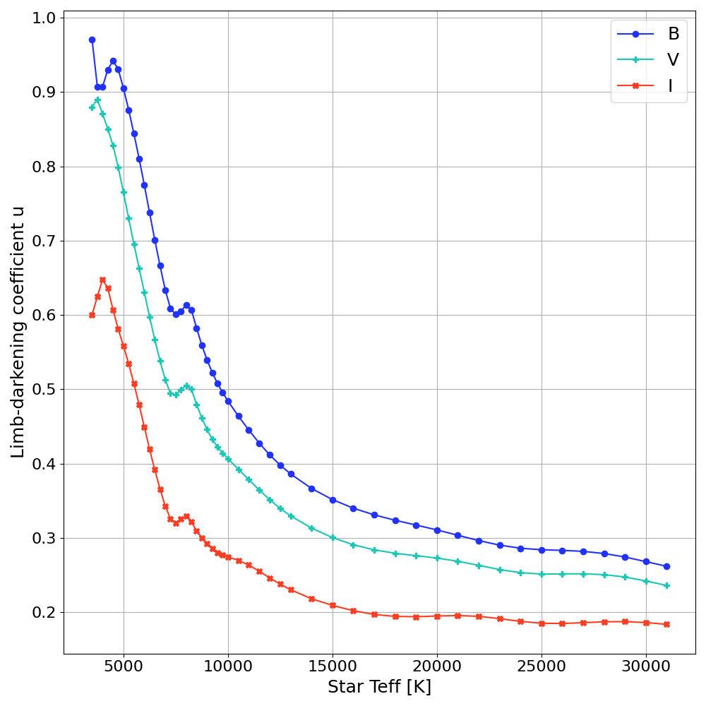
Limb-darkening coefficients appropriate to the passbands used in observations can be found in published tables e.g. Claret et al. 2011. Data on Vizier
Further reading
The Lens Plane
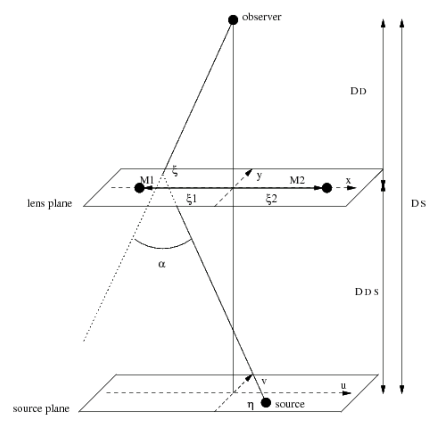
A binary lens has two masses, M1 & M2.
The lens plane coordinate system (x,y) is oriented so that the x-axis passes through the projection of the masses onto the lens plane, with the origin at the central point between the two lens masses.
Both are considered to be at distance DL from the observer, their separation being relatively small.
The Source Plane
The source plane coordinate system, (u,ν), has its origin at the point where the optical axis intersects the source plane.
The optical axis is the line from the observer through the mid-point between the lens masses, so the coordinate system is lens-centric.
Deflection of light by multiple lenses
Each mass deflects a light ray from the source by angle α = 4GM/c2b.
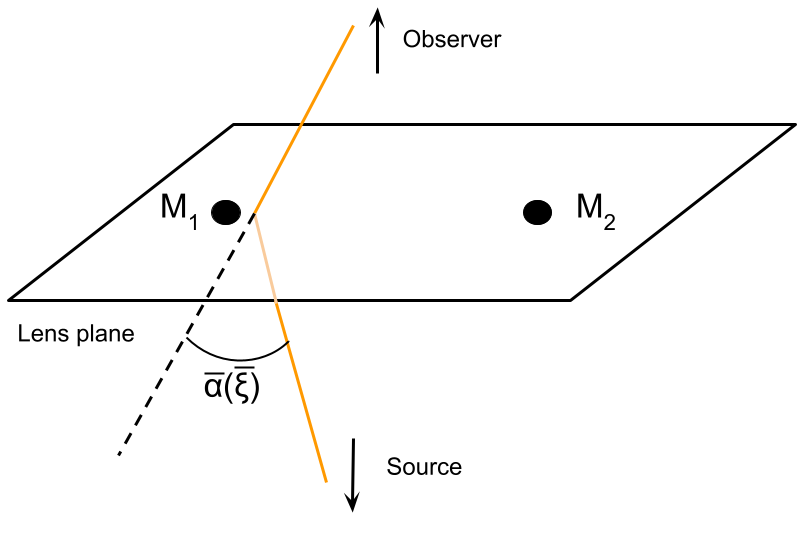
The total deflection is the vector sum of the deflections by each mass.
E.g. a ray which intersects the lens plane at ξ = (x1, y1), has a total deflection for a lens with i = 1 - n masses of:
$$\bar{\alpha}(\bar{\xi}) = \sum_{i}\left( \frac{4GM_{i}}{c^{2}}\frac{\bar{\xi} - \bar{\xi_{i}}}{|\bar{\xi} - \bar{\xi_{i}}|^{2}}\right),$$
The Binary Lens Equation
We now write the lens equation in a form relating the light ray origin in the source plane (η(u,ν)) to the total deflection angle:
$$\bar{\eta} = \bar{\xi}\frac{D_{S}}{D_{L}} - D_{LS}\bar{\alpha}(\bar{\xi}),$$By substituting, we get:
$$\frac{\bar{\eta}}{D_{S}} = \frac{\bar{\xi}}{D_{L}} - \frac{4GM_{1}}{c^{2}}\frac{\bar{\xi} - \bar{\xi_{1}}}{|\bar{\xi} - \bar{\xi_{1}}|^{2}}\frac{D_{LS}}{D_{S}} - \frac{4GM_{2}}{c^{2}}\frac{\bar{\xi} - \bar{\xi_{2}}}{|\bar{\xi} - \bar{\xi_{2}}|^{2}}\frac{D_{LS}}{D_{S}},$$The Binary Lens Equation
This is simplified by declaring:
| $$\bar{w}(u,\nu) = \frac{\bar{\eta}}{D_{S}},$$ | $$\bar{z}(x,y) = \frac{\bar{\xi}}{D_{L}},$$ | $$m_{i} = \frac{4GM_{i}D_{LS}D_{L}}{c^{2}D_{S}},$$ |
and we arrive at:
$$\bar{w} = \bar{z} - m_{1}\frac{\bar{z} - \bar{z_{1}}}{|\bar{z} - \bar{z_{1}}|^{2}} - m_{2}\frac{\bar{z} - \bar{z_{2}}}{|\bar{z} - \bar{z_{2}}|^{2}},$$Mapping between the lens and source planes
This represents a mapping between the source and lens planes:
A light ray from point w̄(u,ν) in the source plane will hit the lens plane at z̄(x,y).
But we are most interested in extracting the locations of the source images in the lens plane geometry.
Locating the source images in the lens plane
As before, solving the binary lens equation gives us the location of the source images.
To achieve this, its convenient to write the lens equation in complex notation
| $$w = z - m_{1}\frac{1}{\bar{z} - \bar{z_{1}}} - m_{2}\frac{1}{\bar{z} - \bar{z_{2}}},$$ | $$w = u + i\nu,$$ | $$z = x + iy,$$ |
where w, z are complex numbers and z̄ is the complex conjugate of z.
Solving this equation requires complex root-finding techniques explored in detail by Schneider & Weiss (1986).
Source Images
Solving this expression for z̄ and substituting, we get (for a binary lens):
$$z = w + \sum_{i=1,2}m_{i}\left[\bar{w} - \bar{z_{i}} + \sum_{k=1,2}m_{k}(z - z_{k})^{-1}\right]^{-1}$$Number of real solutions = number of images of the source
This expression generates a polynomial equation in z of order (n2 + 1), where n is the number of lensing masses.
For a binary lens, there are up to 5 solutions, of which either 3 or 5 may be real, depending on the lens-source projected separation.
Source Images - key takeaways
- Number of images scales with the number of lenses
- Not all solutions are real → not all images exist all the time
- Number and location of images changes with the lens-source projected separation
Magnification for a binary lens
Recall that magnification is the ratio of the lensed/unlensed total image area.
$$A = \left|det\frac{d \alpha}{d \theta} \right|^{-1}$$
Single lens
$$A = \left| det \frac{\partial\bar{w}(u,\nu)}{\partial\bar{z}(x,y)} \right|^{-1},$$
Binary lens
I.e. we calculate the inverse of the area distortion of the lens mapping.
Magnification for a binary lens
The total amplification is given by the sum of the magnification of each image i:
$$A = \sum_{i=1}^{n}A_{i} = \sum_{i=1}^{n}|\det J|^{-1},$$where J is the Jacobian matrix:
$$J = \begin{bmatrix} \frac{\partial u}{\partial x} & \frac{\partial u}{\partial y} \\ \frac{\partial \nu}{\partial x} & \frac{\partial \nu}{\partial y} \end{bmatrix}$$Caustics
As the source moves behind the binary lens, there are certain positions in the source plane for which the resulting Jacobian determinant drops to zero.
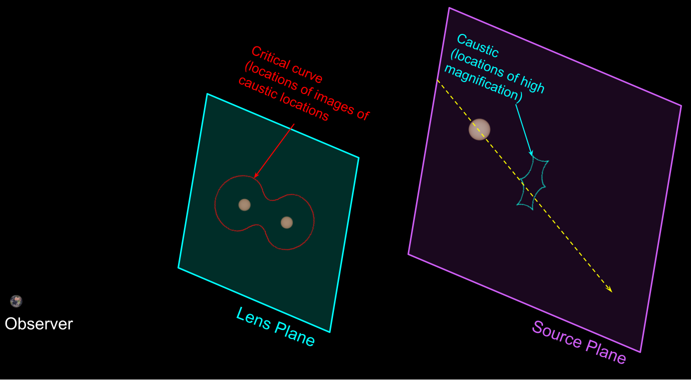
These positions form spikey structures, known as 'caustics'.
Theoretically, as the source crosses these structures, the magnification becomes infinite (curtailed by finite source effects).
Critical Curves
Applying the lens equation, the positions of the caustic in the source plane can be mapped into the lens plane geometry - resulting in graceful curves known as 'critical curves'.
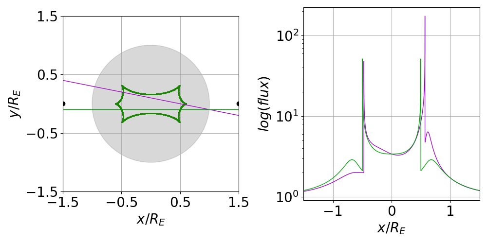
Caustics and lightcurve structure
Number of Lensed Images
- Outside the caustic: 3 images (1 outside and 2 inside the critical curve)
- 2 images exist within the caustic region (1 outside and 1 inside)
- Caustic curve = maximum magnifcation; inside it the magnification can drop
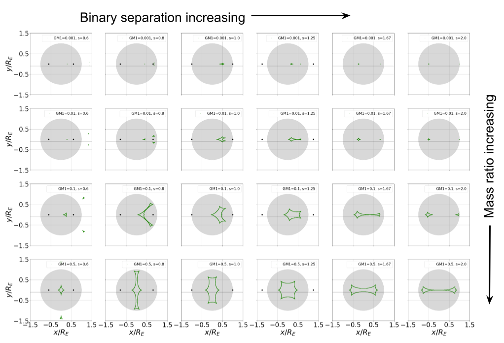
Caustic variety
A wide variety of caustic structures are possible, depending on:
- binary mass ratio
- binary separation
- lens masses' relative angular separation from the source
This simulation has the same parameters as the last one, but M1=0.1, M2=0.9, rather than equal masses
Caustics and Source Trajectories
The source can take any trajectory, relative to the lens geometry, so the lightcurve for the same binary lens can look quite different depending on the angle of incidence.
Planetary caustics
Any binary lens will produce caustics.
Provided the source has a favourable trajectory, even an extreme mass ratio binary like a planetary system will produce a detectable magnification.
This makes microlensing uniquely sensitive to even low mass planetary companions.